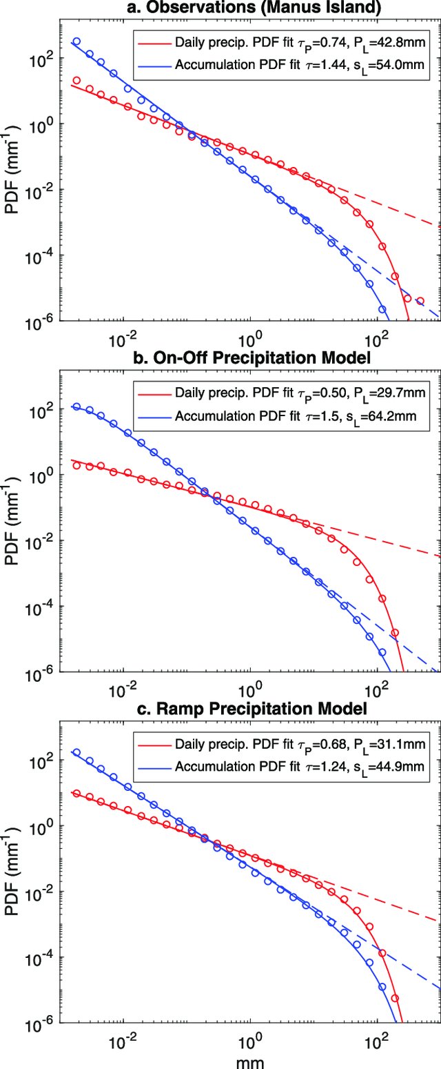
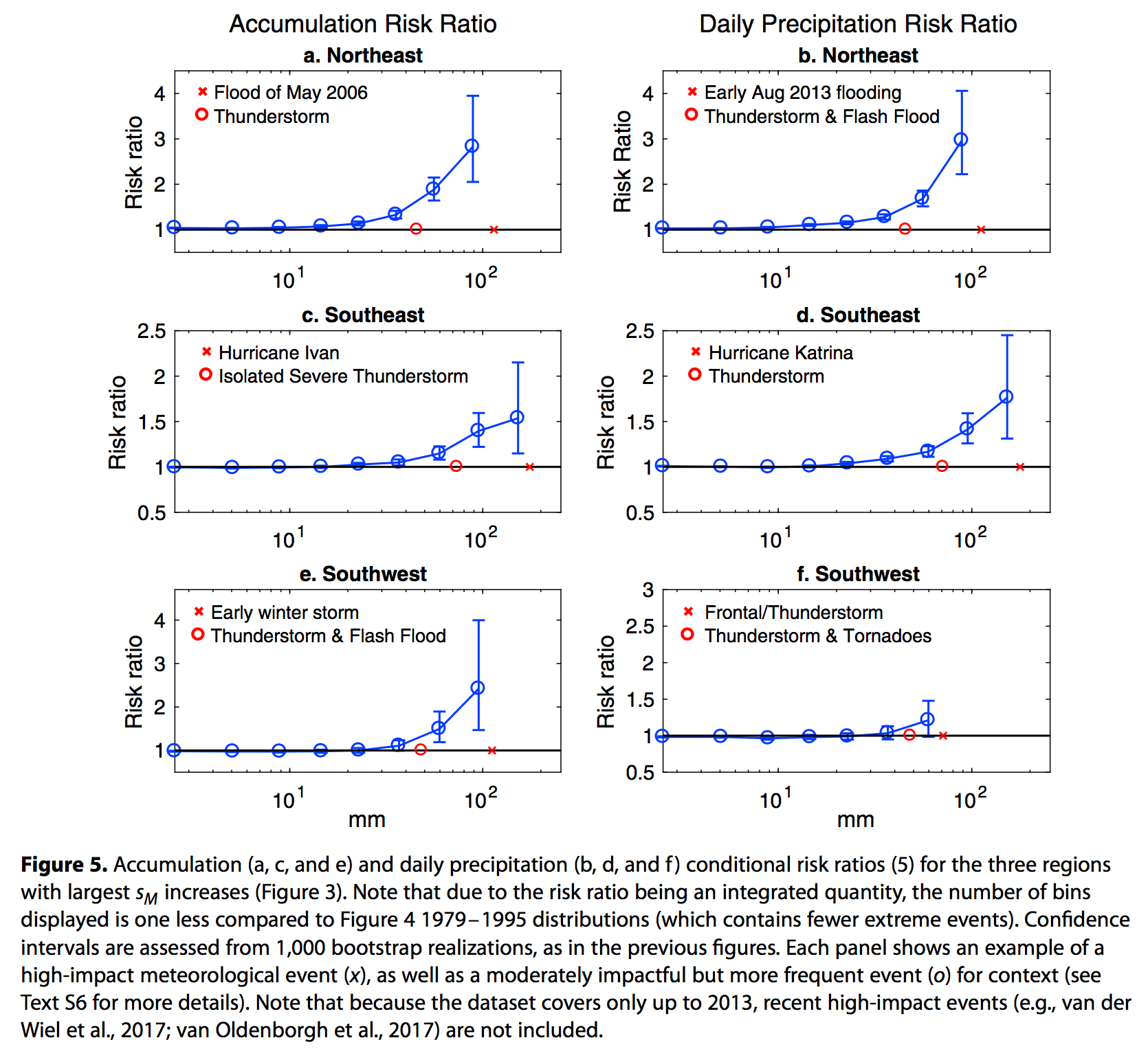
Precipitation accumulations, integrated over rainfall events, are investigated using hourly data across continental China during the warm season (May–October) from 1980 to 2015. Physically, the probability of precipitation accumulations drops slowly with event size up to an approximately exponential cutoff scale s_L where probability drops much faster. Hence s_L can be used as an indicator of high accumulation percentiles (i.e., extreme precipitation accumulations). Overall, the climatology of s_L over continental China is about 54 mm. In terms of cutoff changes, the current warming stage (1980–2015) is divided into two periods, 1980–97 and 1998–2015. We find that the cutoff in 1998–2015 increases about 5.6% compared with that of 1980–97, with an average station increase of 4.7%. Regionally, s_L increases are observed over East China (10.9% ± 1.5%), Northwest China (9.7% ± 2.5%), South China (9.4% ± 1.4%), southern Southwest China (5.6% ± 1.2%), and Central China (5.3% ± 1.0%), with decreases over North China (−10.3% ± 1.3%), Northeast China (−4.9% ± 1.5%), and northern Southwest China (−3.9% ± 1.8%). The conditional risk ratios for five subregions with increased cutoff s_L are all greater than 1.0, indicating an increased risk of large precipitation accumulations in the most recent period. For high precipitation accumulations larger than the 99th percentile of accumulation s₉₉, the risk of extreme precipitation over these regions can increase above 20% except for South China. These increases of extreme accumulations can be largely explained by the extended duration of extreme accumulation events, especially for “extremely extreme” precipitation greater than s₉₉.

Chang, M., B. Liu, C. Martinez-Villalobos, G. Ren, S. Li, and T. Zhou, 2020: Changes in Extreme Precipitation Accumulations during the Warm Season over Continental China. J. Climate, 33, 10799–10811, https://doi.org/10.1175/JCLI-D-20-0616.1

The probability distribution of daily precipitation intensities, especially the probability of extremes, impacts a wide range of applications. In most regions this distribution decays slowly with size at first, approximately as a power law with an exponent between 0 and −1, and then more sharply, for values larger than a characteristic cutoff scale. This cutoff is important because it limits the probability of extreme daily precipitation occurrences in current climate. There is a long history of representing daily precipitation using a gamma distribution—here we present theory for how daily precipitation distributions get their shape. Processes shaping daily precipitation distributions can be separated into nonprecipitating and precipitating regime effects, the former partially controlling how many times in a day it rains, and the latter set by single-storm accumulations. Using previously developed theory for precipitation accumulation distributions—which follow a sharper power-law range (exponent < −1) with a physically derived cutoff for large sizes—analytical expressions for daily precipitation distribution power-law exponent and cutoff are calculated as a function of key physical parameters. Precipitating and nonprecipitating regime processes both contribute to reducing the power-law range exponent for the daily precipitation distribution relative to the fundamental exponent set by accumulations. The daily precipitation distribution cutoff is set by the precipitating regime and scales with moisture availability, with important consequences for future distribution shifts under global warming. Similar results extend to different averaging periods, providing insight into how the precipitation intensity distribution evolves as a function of both underlying physical climate conditions and averaging time.

Martinez-Villalobos, C. and J.D. Neelin, 2019: Why Do Precipitation Intensities Tend to Follow Gamma Distributions?. J. Atmos. Sci., 76, 3611–3631, https://doi.org/10.1175/JAS-D-18-0343.1

https://journals.ametsoc.org/doi/full/10.1175/JAS-D-18-0343.1

 

 

 

Previous studies indicate an asymmetry in the amplitude and persistence of El Niño (EN) and La Niña (LN) events. We show that this observed EN‐LN asymmetry can be captured with a linear model driven by correlated additive and multiplicative (CAM) noise, without resorting to a deterministic nonlinear model. The model is derived from 1‐month lag statistics taken from monthly sea surface temperature (SST) data sets spanning the twentieth century, in an extension of an empirical‐dynamical technique called Linear Inverse Modeling. Our results suggest that noise amplitudes tend to be stronger for EN compared to LN events, which is sufficient to generate asymmetry in amplitude and also produces more persistent LN events on average. These results establish a null hypothesis for EN‐LN asymmetry and suggest that strong EN events may not be more predictable that what can be accounted for by a multivariate linear system driven by CAM noise.

C., Martinez‐Villalobos, Newman, M., Vimont, D. J., Penland, C., & Neelin, J. D. ( 2019). Observed El Niño‐La Niña asymmetry in a linear model. Geophysical Research Letters, 46, 9909-9919. https://doi.org/10.1029/2019GL082922

https://agupubs.onlinelibrary.wiley.com/doi/10.1029/2019GL082922

Precipitation accumulations, integrated over precipitation events in hourly data, are examined from 1979 to 2013 over the contiguous United States during the warm season (May–October). As expected from theory, accumulation distributions have a characteristic shape, with an approximate power law decrease with event size followed by an exponential drop at a characteristic cutoff scale s_L for each location. This cutoff is a predictor of the highest accumulation percentiles and of a similarly defined daily precipitation cutoff P_L. Comparing 1997–2013 and 1979–1995 periods, there are significant regional increases in s_L in several regions. This yields distribution changes that are weighted disproportionately toward extreme accumulations. In the Northeast, for example, risk ratio (conditioned on occurrence) for accumulations larger than 109 mm increases by a factor of 2–4 (5th–95th). These changes in risk ratio as a function of size, and connection to underlying theory, have counterparts in the observed daily precipitation trends.

Martinez‐Villalobos, C., & Neelin, J. D. (2018). Shifts in precipitation accumulation extremes during the warm season over the United States. Geophysical Research Letters, 45, 8586–8595. https://doi.org/10.1029/2018GL078465

https://agupubs.onlinelibrary.wiley.com/doi/full/10.1029/2018GL078465

The most commonly used version of a linear inverse model (LIM) is forced by state-independent noise. Although having several desirable qualities, this formulation can only generate long-term Gaussian statistics. LIM-like systems forced by correlated additive–multiplicative (CAM) noise have been shown to generate deviations from Gaussianity, but parameter estimation methods are only known in the univariate case, limiting their use for the study of coupled variability. This paper presents a methodology to calculate the parameters of the simplest multivariate LIM extension that can generate long-term deviations from Gaussianity. This model (CAM-LIM) consists of a linear deterministic part forced by a diagonal CAM noise formulation, plus an independent additive noise term. This allows for the possibility of representing asymmetric distributions with heavier- or lighter-than-Gaussian tails. The usefulness of this methodology is illustrated in a locally coupled two-variable ocean–atmosphere model of midlatitude variability. Here, a CAM-LIM is calculated from ocean weather station data. Although the time-resolved dynamics is very close to linear at a time scale of a couple of days, significant deviations from Gaussianity are found. In particular, individual probability density functions are skewed with both heavy and light tails. It is shown that these deviations from Gaussianity are well accounted for by the CAM-LIM formulation, without invoking nonlinearity in the time-resolved operator. Estimation methods using knowledge of the CAM-LIM statistical constraints provide robust estimation of the parameters with data lengths typical of geophysical time series, for example, 31 winters for the ocean weather station here.

Martinez-Villalobos, C., D.J. Vimont, C. Penland, M. Newman, and J.D. Neelin, 2018: Calculating State-Dependent Noise in a Linear Inverse Model Framework. J. Atmos. Sci., 75, 479–496, https://doi.org/10.1175/JAS-D-17-0235.1

https://journals.ametsoc.org/doi/abs/10.1175/JAS-D-17-0235.1

A theoretical framework is developed for understanding the transient growth and propagation characteristics of thermodynamically coupled, meridional mode–like structures in the tropics. The model consists of a Gill–Matsuno-type steady atmosphere under the long-wave approximation coupled via a wind–evaporation–sea surface temperature (WES) feedback to a “slab” ocean model. When projected onto meridional basis functions for the atmosphere the system simplifies to a nonnormal set of equations that describes the evolution of individual sea surface temperature (SST) modes, with clean separation between equatorially symmetric and antisymmetric modes. The following major findings result from analysis of the system: 1) a transient growth process exists whereby specific SST modes propagate toward lower-order modes at the expense of the higher-order modes; 2) the same dynamical mechanisms govern the evolution of symmetric and antisymmetric SST modes except for the lowest-order wavenumber, where for symmetric structures the atmospheric Kelvin wave plays a critically different role in enhancing decay; and 3) the WES feedback is positive for all modes (with a maximum for the most equatorially confined antisymmetric structure) except for the most equatorially confined symmetric mode where the Kelvin wave generates a negative WES feedback. Taken together, these findings explain why equatorially antisymmetric “dipole”-like structures may dominate thermodynamically coupled ocean–atmosphere variability in the tropics. The role of nonnormality and the role of realistic mean states in meridional mode variability are discussed.

Martinez-Villalobos, C. and D.J. Vimont, 2017: An Analytical Framework for Understanding Tropical Meridional Modes. J. Climate, 30, 3303–3323,https://doi.org/10.1175/JCLI-D-16-0450.1

https://journals.ametsoc.org/doi/abs/10.1175/JCLI-D-16-0450.1

This study uses a simple linear coupled model to investigate the role of the WES feedback and ITCZ mean states in meridional mode variability. Optimal structures that maximize transient growth are calculated for mean states characteristic of boreal spring and boreal fall in the tropical Atlantic. During boreal spring the leading optimal structure is a zonal mode that propagates westward and does not resemble the observed meridional mode. In contrast, the leading optimal structure during fall is a sea surface temperature (SST) monopole over the Northern Hemisphere (NH) that propagates equatorward and westward and that closely matches meridional mode variability during this season. It is found that the boreal fall optimal growth greatly exceeds growth of the corresponding optimal during boreal spring, despite the observed boreal spring peak in Atlantic meridional mode variance.

Sensitivity studies are used to explore the role of Northern or Southern Hemisphere initial conditions, ITCZ width, and ITCZ location in meridional mode growth and structure. It is found that growth is favored (i) for optimal structures that originate in the Northern Hemisphere, especially for boreal fall mean states; (ii) for symmetric mean states, equatorially symmetric structures maximize growth under narrow ITCZ configurations, and antisymmetric structures maximize growth under wider ITCZ configurations; and (iii) for antisymmetric mean states (and realistic ITCZ width), growth is maximized when the ITCZ is located off of the equator. The implications of these findings are discussed.

Martinez-Villalobos, C. and D.J. Vimont, 2016: The Role of the Mean State in Meridional Mode Structure and Growth. J. Climate, 29, 3907–3921,https://doi.org/10.1175/JCLI-D-15-0542.1

https://journals.ametsoc.org/doi/full/10.1175/JCLI-D-15-0542.1

The semihadronic tau decay width allows a clean extraction of the strong coupling constant at low energies. We present a modification of the standard “contour-improved” method based on a derivative expansion of the Adler function. The new approach has some advantages compared to contour-improved perturbation theory. The renormalization scale dependence is weaker by more than a factor of 2 and the last term of the expansion is reduced by about 10%, while the renormalization scheme dependence remains approximately equal. The extracted QCD coupling at the tau mass scale is by 2% lower than the contour-improved value. We find ${\mathrm{\alpha \_\{s\}}}^{}\left({\mathrm{M\_\{Z\}^\{2\}}}^{}\right)=0.1211\pm 0.0010$.

G. Cvetič, M. Loewe, C. Martinez and C. Valenzuela, Phys. Rev. D 82, 093007. DOI: https://doi.org/10.1103/PhysRevD.82.093007

https://journals.aps.org/prd/abstract/10.1103/PhysRevD.82.093007